The Strava global heatmap is a really cool way of visualizing the popularity of cycling and running routes around the world. It’s also interesting challenge on two fronts: efficiently building the heatmap from millions of activities, and efficiently serving the map tiles.
Building the heatmap
Previously, the heatmap was created with C code that accessed activities with individual S3 requests. The latest version is built on Apache Spark to be parallelizable at every stage. It uses a “Spark/S3/Parquet data warehouse” for data storage – Parquet being a columnar storage format that’s built for doing distributed jobs, working on top of the Hadroop filesystem.
Data is filtered to remove data that is likely the result of non-biking or running activities. It’s also normalized for velocity - sitting at a traffic light won’t produce more data points than going 20mph on a bike.
The computation is parallelized on a per-tile basis. Since the primitives drawn are paths rather than points, this means that each path must be resampled to fit inside a single tile.
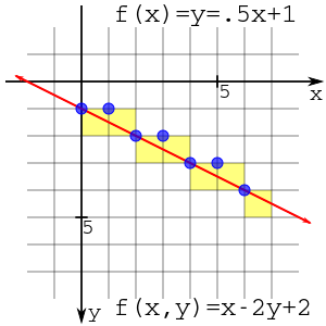
Line drawing is done using Bresenham’s line algorithm for efficiency. A first stab at a line-drawing might involve looping from the origin the endpoint and adding the slope on each iteration. But this involves float multiplication, which is unnecessary when we’re dealing with discrete tiles. Bresenham’s algorithm uses only integer addition/subtraction and bitshifting, where the steps are as follows:
    d = 2*dy - dx
    y = y_start

    for x in range(x_start, x_end):
        plot(x, y)
    		if d > 0:
    			y = y + 1
    			d = d - 2*dx
    		d = d + 2*dy
With dx = 6, dy =3 ( slope of .5), we have the following pattern:
| iteration | d (before) | y (before) |
|---|---|---|
| 0 | 0 | 0 |
| 1 | 0 + 6 = 6 | 0 |
| 2 | 6 - 12 + 6 = 0 | 1 |
| 3 | 0 + 6 = 6 | 1 |
Whatever files are currently being processed are stored as nxn matrices, then compressed and written to disk when done.
Normalization
If the samples in a given pixel were linearly mapped to colors, this would result in only the most popular areas being visible (which might have 100x the number of visitors as a less popular area). For normalization, they use the CDF of the pixel values, so that the median pixel is half as strong as the most-traversed pixel.
The CDF is calculated on a per-tile level, but includes the surrounding tiles as well. This ensures that there’s a smooth transition between tiles - otherwise, a route might suddenly disappear when it goes from a less popular tile to a more popular one.
Each pixel is actually bilinearly interpolated from the CDFs of its surrounding pixels. It’s not clear how this affects parallelization at the per-tile level.
Serving tiles
Tiles at different more zoomed out zoom levels are greater simply by sampling the lower zoom levels.
Tiles are stored on S3 as raw byte values, corresponding to values of the 8-bit color map. These are then are converted to pngs at request time (and cached via their CDN).